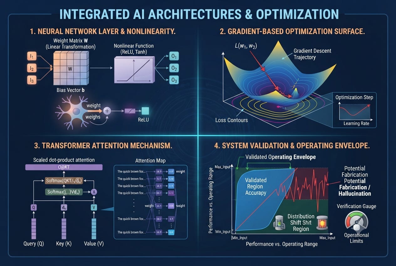
Artificial intelligence works by routing data through layered mathematical functions whose parameters get tuned through calculus based optimization, a process that used 415 terawatt hours of electricity worldwide in 2024. Every input, whether a sentence of text, a photograph, or a sensor reading, is first converted into a list of numbers. Those numbers pass through many layers of arithmetic, each layer shaped by parameters learned from data rather than programmed by hand. A training procedure repeatedly compares the system’s output to a known correct answer and adjusts every parameter using a calculus technique called backpropagation, in much the same way an engineer uses adjoint sensitivity analysis to trace how a design change ripples backward through a coupled physical model. Once training stops, the same fixed arithmetic runs forward only, at a fraction of the original computational cost, to produce predictions on data it has never encountered.
What Mathematical Operation Actually Happens Inside a Neural Network?
A single artificial neuron performs one operation: it multiplies each incoming number by a weight, adds those products together with a bias term, and passes the sum through a nonlinear function. The nonlinear step matters. Without it, stacking layers would collapse into a single linear transformation, no more expressive than one matrix multiplication no matter how many layers were added. With a nonlinearity such as the rectified linear unit, which simply outputs zero for any negative input and passes positive input through unchanged, a network of stacked layers can approximate almost any continuous function given enough neurons, a result formalized in the universal approximation theorems of the late 1980s and early 1990s.
For an engineer trained in linear systems, the closest analogy is a block diagram in which each block applies a gain and then a saturation nonlinearity, similar to the transfer function of an amplifier stage that clips at its rails. A neural network layer is that block diagram generalized to thousands of inputs and thousands of outputs simultaneously, represented as a matrix multiplication followed by an elementwise nonlinear function, and a full network is dozens or hundreds of these blocks connected in series. The parameters inside those matrices, the weights and biases, are the only quantities the network actually learns. A modest network with three layers of one thousand neurons each already contains roughly two million such weighted connections. A large language model released in 2020 disclosed 175 billion parameters, and systems built three years later used training computation on the order of one hundred times greater still.
Modern networks also commonly include a residual connection, a direct path that adds a layer’s input back to its output alongside the normal calculation, introduced in the mid 2010s to solve a practical training problem: without that direct path, gradients computed during backpropagation tend to shrink toward zero as they travel backward through many layers, leaving the earliest layers of a deep network barely updated at all. A residual connection functions much like a feedback path around a control block: it guarantees a signal can pass through a stage largely unmodified when the learned transformation at that stage is not yet useful, which is part of why networks with over one hundred layers became trainable at all.
Nothing about this arithmetic encodes physical law, chemical kinetics, or a governing differential equation. The network has no built in notion of conservation of mass, momentum, or energy unless a designer explicitly adds a penalty term to enforce one. It is, at its core, a very large adjustable curve fit, and every claim about what the system understands has to be evaluated against that fact.
How Does a Neural Network Learn From Data?
Training begins by setting every weight to a small random number. The network then performs a forward pass: it takes a training example, pushes it through every layer, and produces an output. That output is compared against the known correct answer using a loss function, a single number that measures how wrong the prediction was. The learning step is where calculus enters. Backpropagation applies the chain rule layer by layer, moving backward from the loss through every weight in the network, to compute exactly how much a small change in each individual weight would change the loss. This produces a gradient: a vector, with one entry per weight, pointing in the direction of steepest increase in error.
Gradient descent then moves every weight a small step in the opposite direction, the direction that reduces the loss, and the cycle repeats on the next training example or batch of examples. The size of that step is called the learning rate, and it behaves exactly like an under relaxation factor in an iterative computational fluid dynamics solver: set it too high and the solution oscillates or diverges, set it too low and the calculation takes an impractical number of iterations to converge. Most modern training uses stochastic gradient descent, updating weights on small random batches of data rather than the full dataset at once, which trades a noisier gradient estimate for the ability to take far more update steps per hour of computation.
Engineers who work with adjoint methods for shape optimization, whether tuning a turbine blade profile or a reactor core loading pattern, will recognize backpropagation immediately. Both techniques solve the same underlying problem: given a scalar objective that depends on an enormous number of design variables, compute the sensitivity of that objective to every variable in a single backward sweep, rather than perturbing each variable one at a time and rerunning the entire forward calculation. The difference is scale and purpose. An adjoint solver in aerospace design might handle thousands of variables tied to a physical mesh. Backpropagation in a large model routes gradients through billions of weights with no physical mesh underneath them at all, and the resulting optimization surface is nonconvex, meaning gradient descent finds a local minimum with no guarantee it is the best possible one and no closed form check available to confirm the answer, unlike solving a linear structural system where the solution can be verified against a known stiffness matrix.
What Is a Loss Function, and How Does It Work Like an Objective Function in Engineering Optimization?
A loss function is the quantity training tries to minimize, and it plays exactly the role an objective function plays in topology optimization or core design: it converts a design goal into a single differentiable number. For predicting a continuous quantity, the loss is often mean squared error, the average of the squared difference between prediction and target, the same quantity minimized in ordinary least squares curve fitting since the eighteenth century. For classification tasks, including next word prediction in a language model, the loss is typically cross entropy, which measures the distance between the model’s predicted probability distribution over possible answers and the actual correct answer.
Minimizing loss on the training data alone is not the actual goal. A model that perfectly memorizes every training example, achieving near zero loss on data it has already seen, often performs poorly on new data it has never seen, a failure mode called overfitting. This is the direct analog of designing a component to satisfy exactly one calibration load case while ignoring the full distribution of loads it will actually see in service. Engineers address that risk with safety factors and design margins across a range of expected conditions. Model training addresses the analogous risk with techniques such as weight decay, which adds a penalty for large parameter values the same way a mass penalty discourages an optimizer from adding unnecessary material, and dropout, which randomly disables a fraction of neurons during each training step to prevent the network from relying too heavily on any single pathway, forcing redundancy into the learned representation the way a designer might deliberately avoid a single point of failure in a control system.
Why Did AI Systems Move From Recurrent Networks to the Transformer Architecture?
Before 2017, the dominant approach to processing sequences of text used recurrent neural networks, which read one word at a time and carried a running internal state forward to the next step, similar to a time marching finite difference solver in which the state at each time step depends entirely on the state computed at the previous step. That sequential dependency created a real computational bottleneck: because step ten cannot start until step nine finishes, the calculation cannot be spread efficiently across many parallel processors, no matter how many are available.
In 2017, researchers introduced an architecture built around a mechanism called attention, which allows every position in a sequence to be processed against every other position simultaneously rather than one step at a time, closer to solving a global system across an entire domain at once than marching forward one grid point at a time. Removing the sequential bottleneck meant the underlying matrix operations could be distributed across thousands of processors running in parallel, and that single change is largely responsible for the growth in model size seen over the following years. Independent analysis published in 2024 found that the computational budget used to train the largest disclosed models grew at a rate of four to five times per year between 2010 and 2024, reaching training runs on the order of ten to the twenty fifth power floating point operations by 2023, roughly one hundred times the computation used to train the 175 billion parameter model released in 2020.
This architecture, generally called the transformer, is now the basis for nearly every large language model in commercial use, as well as many systems that process images, audio, and even protein sequences, because the same parallel attention mechanism generalizes to any data that can be represented as a sequence of tokens.
What Is Attention, and How Is It Similar to a Weighted Sensor Fusion Calculation?
Attention computes, for every element in a sequence, how much weight to give every other element when forming an updated representation of that element. Mechanically, each token is projected into three vectors called a query, a key, and a value. The query for one token is compared against the key of every other token using a dot product, producing a raw similarity score for each pair. Those scores are normalized with a function called softmax, which converts them into positive weights that sum to one, and the token’s updated representation becomes the weighted sum of every other token’s value vector using those weights.
An engineer working with state estimation will recognize the shape of this calculation. A Kalman filter combines measurements from multiple sensors by weighting each one according to its estimated reliability, giving more influence to a low noise sensor and less to a noisy one, rather than averaging every measurement equally. Attention performs a conceptually similar weighting, except the weights are not derived from a known noise covariance; they are learned from data and recomputed fresh for every single input, which is why the same attention mechanism can decide, in one sentence, that a pronoun should draw most of its meaning from a noun several words earlier, and in the next sentence draw it from a noun that immediately precedes it. Modern architectures run many attention calculations in parallel, called multiple heads, each learning to track a different kind of relationship in the data, comparable to running several independently tuned filters, each sensitive to a different frequency band or failure signature, and combining their outputs into one estimate.
How Is a Large Language Model Actually Trained, From Raw Text to a Working System?
The process begins with tokenization: raw text is broken into subword units, and each unit is mapped to an integer identifier from a fixed vocabulary, typically tens of thousands of entries. Each integer is then converted into an embedding, a learned vector of a few thousand numbers that gives the token a position in a high dimensional space where tokens with related meaning end up closer together. These embeddings, not the raw text, are what the network actually processes.
The primary training objective for most current systems is simple to state: given every token so far in a passage, predict the next one, and adjust every parameter through backpropagation and gradient descent to make that prediction closer to the token that actually appeared next in the training text. This objective is repeated across trillions of tokens drawn from text, code, and other sources, at a computational cost measured in the tens of millions of dollars for the largest systems as of the early 2020s. Because the objective requires no manually labeled answer for each example, only the next word in text that already exists, it is described as self supervised, and it is what allows training at this scale in the first place.
A second stage typically follows pretraining. The base model, having learned to predict plausible continuations of text, is then adjusted on a smaller, carefully curated set of examples showing the kind of behavior developers want, questions paired with helpful answers, for instance, and further refined using feedback, either from human reviewers or from a separate model trained to imitate human preference judgments, in a process commonly called reinforcement learning from feedback. This second stage does not add new factual knowledge to the system in any meaningful sense. It reshapes how the model uses the knowledge already encoded in its parameters from pretraining, closer to recalibrating a sensor’s output curve than to installing a new sensor.
It bears restating plainly for an audience trained in physical modeling: none of this involves the system checking a fact against an external source of truth at the moment it generates a response. The entire system is a statistical model of which sequence of tokens is likely to follow which, built from an enormous amount of prior text. That is a categorically different kind of model from a symbolic reasoning engine that manipulates explicit logical rules, and the distinction explains a great deal about where these systems succeed and where they fail.
What Is Fine Tuning, and How Is It Like Adapting a Validated Instrument for a New Application?
Training a large model from scratch is rarely how a specific product gets built. Instead, a developer typically starts from a base model that already went through the full pretraining process described above, at the cost of tens of millions of dollars in computation, and adapts that base model to a narrower task using a much smaller dataset and a much smaller computational budget, often a tiny fraction of one percent of the original training cost. This is called fine tuning, and it works because most of the general capability the model needs, grammar, broad world knowledge, basic reasoning patterns, was already captured during pretraining, so the fine tuning stage only has to adjust the model’s behavior for the specific application rather than teach it from nothing.
An engineer who calibrates a general purpose instrument, a pressure transducer or an accelerometer, for a specific installation before deploying it will recognize the underlying logic. The instrument’s core physics do not change between installations. What changes is a smaller set of calibration constants tuned for the particular operating range and mounting conditions of that one installation. Fine tuning plays a similar role for a trained model: the underlying parameters that encode general language ability stay largely fixed, while a comparatively small adjustment reshapes the model for one narrower purpose, whether that purpose is answering customer support questions for one company’s products or reviewing contracts for one specific area of law.
A related technique called retrieval augmentation addresses a different limitation directly. Rather than retraining the model to memorize new facts, the system instead searches an external document collection at the moment a query arrives, retrieves the most relevant passages, and inserts that retrieved text directly into the model’s input alongside the original question, so the model’s response is generated with the actual source material in front of it rather than relying solely on whatever it absorbed during training months or years earlier. This is the closest analog in current systems to checking a result against an external reference, and it measurably reduces, though does not eliminate, the fabrication problem described later in this piece.
How Does a Trained Model Generate a Response One Word at a Time?
Everything described so far explains how a model is built. Generating an actual response, called inference, is a separate and much simpler calculation performed after training is complete. The model does not produce a full answer in one step. It produces a probability distribution over every possible next token given everything written so far, selects one token from that distribution, appends it to the growing text, and repeats the entire calculation again with the new, longer input, one token at a time, in a process called autoregressive decoding.
How a token gets selected from that probability distribution is itself an adjustable design choice, not a fixed rule. Always picking the single most likely next token produces flat, repetitive, and predictable text. Introducing controlled randomness, governed by a parameter commonly called temperature, allows lower probability tokens to be selected some of the time, which produces more varied and often more natural output at the cost of occasionally selecting a less probable, and therefore potentially less accurate, continuation. This is a direct, quantifiable trade off between output variety and output reliability, tuned by a single numerical parameter, similar to adjusting a filter’s cutoff frequency and accepting more noise in exchange for less signal delay.
The model can only consider a limited stretch of prior text at once, called its context window, which for a currently deployed system typically ranges from tens of thousands to several hundred thousand tokens. Every token inside that window gets compared against every other token during the attention calculation described earlier, and the computational cost of that comparison grows with the square of the window’s length, which is why extending how much text a model can consider at once remains an active area of hardware and algorithm development rather than a solved problem.
What Computer Hardware Actually Runs AI Training and Inference?
Neural network training and inference reduce, almost entirely, to matrix multiplication performed over and over at enormous volume. A conventional processor is built to execute a long sequence of different instructions quickly, branching between operations, managing memory, and handling many dissimilar tasks one after another with very low latency on each individual step. A graphics processor takes the opposite design approach: it runs the same simple arithmetic operation across thousands of small cores at once, a design originally built for rendering millions of pixels in parallel that happens to match the repeated multiply and add pattern inside a neural network layer far better than a general purpose processor does.
This is why graphics processors, not conventional processors, became the standard hardware for training. Specialized data center chips built for this purpose, several successive generations of which have been produced since the early 2010s, are now designed less around raw arithmetic speed and more around memory bandwidth, the rate at which numbers can be moved between memory and the arithmetic units doing the multiplying. The arithmetic itself, multiply and add, is trivial. Moving the enormous matrices involved fast enough to keep thousands of arithmetic units continuously supplied with fresh numbers is the actual engineering constraint, comparable to a chemical process where the limiting factor is not reaction kinetics but mass transfer through the piping that feeds the reactor.
A single chip’s memory cannot hold a frontier model’s full set of parameters together with the data needed to train it, so training runs are distributed across clusters of thousands of chips connected by high speed networking, with the model and the dataset split across the cluster the way a large finite element problem gets divided across many processors in parallel computing, each processor handling one portion of the domain and periodically exchanging results with its neighbors. Building and cooling these clusters, not writing the underlying software, is now the primary capital constraint on how large a model an organization can train.
How Much Electricity Does Training and Running These Systems Actually Require?
Global data centers running AI and other digital workloads consumed an estimated 415 terawatt hours of electricity in 2024, about 1.5 percent of world electricity use, a figure that has grown at roughly 12 percent per year since 2017, several times faster than growth in overall global electricity demand. Current projections place that figure near 945 terawatt hours by 2030. One widely circulated industry estimate projects that training a single frontier model by 2027 could require as much as five gigawatts of continuous power, comparable to the output of several large power stations running simultaneously, and that the domestic AI sector as a whole may need on the order of 50 gigawatts of new electric generating capacity by 2028 to keep pace with planned construction.
The electricity mix serving these data centers in 2024 broke down roughly as follows: natural gas supplied about 40 percent, renewable generation about 24 percent, nuclear power about 20 percent, and coal about 15 percent. For an audience with a direct stake in nuclear generation, that 20 percent figure is the practical reason several data center operators have signed long term power purchase agreements directly with nuclear plant operators and pursued licensing for small modular reactors sited near planned data center campuses.
It is worth separating two very different costs. Training a frontier model is a one time expense, extraordinarily energy intensive but bounded: once training finishes, that specific computational cost is not repeated. Inference, running the trained model to answer an individual query, costs far less energy per use, but that small cost is multiplied across billions of queries every day across every deployed system, and the cumulative total is what actually drives long run electricity demand. The comparison an engineer will find familiar is the difference between the energy cost of manufacturing a single unit of equipment and the cumulative energy cost of operating an entire fleet of that equipment for years afterward.
The thermal side of this problem is a mechanical engineering problem as much as an electrical one. A rack of data center chips packed densely enough to train a frontier model in a reasonable amount of time can no longer be cooled adequately with air alone, so newer facilities increasingly use direct liquid cooling, circulating fluid through cold plates mounted directly on each chip, the same underlying heat transfer principle used in a car radiator or a reactor cooling loop, just scaled to remove heat densities that air cooling cannot handle economically at this density. Some of the larger planned data center campuses have accordingly drawn direct comparisons to industrial cooling water demand, which is part of why several proposed sites have been evaluated for water availability with the same seriousness historically reserved for a conventional power plant or an industrial cooling tower installation, rather than treated as an ordinary commercial building.
Why Do AI Systems Fail in Ways a Correctly Designed Engineered System Should Not?
A structural model derived from first principles carries built in physical constraints. Mass balances close. Energy is conserved. A result that violates a known physical law is immediately recognizable as an error. A trained neural network carries no such constraint unless a designer explicitly builds one in, because the model was fit to data, not derived from a governing equation, and it will produce a confident, fluent output for an input far outside anything it was trained on, the same way a regression line will still return a number if extrapolated far past its calibration range, with no internal indicator that the number has become meaningless.
This is the underlying mechanism behind what is commonly called hallucination in language models: the system generates a statistically plausible continuation of text, because that is precisely what it was trained to do, with nothing in its architecture that checks the generated statement against an external source of truth before producing it. The output can be fluent, confident, and entirely fabricated at the same time, because fluency and correctness are governed by different parts of the process, and only fluency is what the training objective directly optimizes.
A second failure mode, distribution shift, occurs when the statistical pattern of real world inputs during deployment differs from the statistical pattern of the training data, even when every individual input looks reasonable on its own. A model that performed well on its test dataset can degrade sharply once deployed against a population of inputs the training data did not represent, comparable to a controller tuned for one operating envelope losing stability once operated outside it. A third failure mode, adversarial fragility, refers to the fact that small, deliberately chosen changes to an input, changes a human observer would barely notice, can produce large and unpredictable changes in a model’s output, a property that would be considered a serious defect in a well conditioned physical system but is a documented characteristic of many trained models as built today.
A concrete illustration ties these three failure modes together. A vision model trained to flag surface defects on machined parts, trained entirely on photographs taken under one lighting setup and one camera angle, can perform very well in validation testing and still fail once installed on an actual production line, because the lighting, camera angle, and part orientation on the floor differ enough from the training photographs that the model is effectively operating in a distribution shift condition without anyone having labeled it that way. The model will not report reduced confidence in that situation. It will report a confident classification either way, correct or not, because nothing in its training taught it to recognize when its own input has moved outside familiar territory. That is the specific property, confident output regardless of whether the input resembles training data, that separates a trained model’s failure behavior from the failure behavior of an instrument that reports an out of range fault when a physical sensor limit is exceeded.
How Should an Engineer Approach Verification and Validation of a System With No Closed Form Model?
Nuclear and mechanical engineering already have a mature answer to the general problem of validating a system that cannot be verified by a single proof of correctness: probabilistic risk assessment, failure modes and effects analysis, and layered defenses that assume any single barrier can fail. That practice transfers directly to AI systems, because a trained model shares the same underlying limitation as any complex system without a closed form governing equation: there is no single calculation an engineer can run to confirm the system will behave correctly across every condition it might encounter.
A federal framework published in January 2023 organizes AI risk management into four functions: govern, map, measure, and manage, a formal structure focused on documenting where a system will be used, testing it across that intended range of use, and monitoring it continuously after deployment rather than treating a single pre deployment test as sufficient. In practice, that means testing across a representative range of operating conditions before deployment, documenting exactly what data trained the system and what its known limitations are, monitoring its outputs after deployment for signs that real world inputs have drifted away from the training distribution, and keeping a human reviewer positioned to catch errors the automated system will not catch on its own, the same layered logic behind defense in depth in reactor safety design.
In reviewing technical disclosures and evaluating patent applications for clients deploying trained models inside safety relevant products, the recurring gap is rarely in the underlying mathematics, which is usually documented in enough detail to satisfy a technical reviewer. The recurring gap is the absence of a bounded operating envelope: a written statement of the specific range of inputs across which the system’s behavior has actually been tested and characterized, the direct equivalent of a safe operating envelope for a pressure vessel. A model without that written envelope has not been validated in any sense an engineer trained on physical systems would recognize, regardless of how accurate its published benchmark scores may be.
What Should an Engineer Outside Computer Science Take From This?
Artificial intelligence, as practiced today, is applied numerical optimization operating on an enormous number of parameters, not deduction from a governing physical law. The mathematics underneath it, matrix multiplication, gradient based optimization, and a weighting mechanism borrowed conceptually from sensor fusion, will already be familiar territory to a mechanical or nuclear engineer, even though the vocabulary surrounding it rarely says so directly. What will not be familiar, and what deserves the same rigor already applied to any other high consequence system, is the absence of a governing equation to catch an error. Treat the training data, the documented operating envelope, and the monitoring plan with the same seriousness given to a stress analysis or a safety case, because nothing else in the system is going to catch a mistake for you.
The next piece in this series examines how the enablement requirement under 35 U.S.C. section 112 applies when a patent specification discloses a trained model instead of a written algorithm, and why a growing number of rejections issued by the mechanical and electrical art units at the patent office in the past year have turned on exactly that missing operating envelope.
Bibliography
Rosenblatt, F. Foundational paper introducing the perceptron, an early trainable model for pattern recognition. Psychological Review, volume 65, 1958.
Rumelhart, D. E., Hinton, G. E., and Williams, R. J. Foundational paper describing the backpropagation algorithm for training multilayer neural networks. Nature, volume 323, 1986.
Krizhevsky, A., Sutskever, I., and Hinton, G. E. Paper describing a deep convolutional neural network that substantially improved image classification accuracy on a large benchmark dataset. Advances in Neural Information Processing Systems, 2012.
Vaswani, A., Shazeer, N., Parmar, N., and coauthors. Paper introducing the transformer architecture and the attention mechanism now used in most large language models. arXiv preprint 1706.03762, 2017.
Brown, T., and coauthors. Paper describing a 175 billion parameter language model and its training methodology. Advances in Neural Information Processing Systems, 2020.
National Institute of Standards and Technology. Artificial Intelligence Risk Management Framework, publication AI 100 1, January 26, 2023.
Sevilla, J., and Roldan, E. Analysis of training compute growth across frontier AI models from 2010 to 2024, including specific compute estimates for major disclosed models. Epoch AI, May 28, 2024.
International Energy Agency. Data center electricity demand estimates and 2030 projections, as synthesized in a Brookings Institution analysis of global electricity demand tied to AI regulatory policy, published 2026.
Lawrence Berkeley National Laboratory. United States data center electricity demand projections through 2028, 2024, as synthesized in the Brookings Institution analysis cited above.
Anthropic. Public projections on frontier model training power requirements and United States AI sector electricity capacity needs, 2024 to 2025, as synthesized in the Brookings Institution analysis cited above.
Congressional Research Service. Data Centers and Their Energy Consumption: Frequently Asked Questions, report R48646, 2025.